Damn, Voxel Data is BIG

I left off the last post with a little question about how many voxels I might need to represent a planet.  There were a few guesses of  4.7810528e+20, 9.8782084e+17 and 10^21 which at first glance seem absurdly large but in fact they were pretty close to the mark.  You see the thing about voxel data is it's big.  Very big.

Apart from the inherent inefficiencies of using GPUs to render voxels with raycasting when they would generally be much happier doing what they were designed for and be rasterising triangles, it's the amount of memory voxel data sets consume that prohibit their use in many scenarios and while that's pretty much accepted wisdom and hardly newsworthy - I thought it might be interesting to just take a moment to put out there some cold hard numbers.

So, how many voxels and therefore of course bytes of storage do you need to render a planet?  The answer as you would expect depends on the fidelity of your representation and your method of storage, but these are my numbers what what they're worth:

To encompass a maximum data set of 25,000 Km cubed I am using 22 levels of detail each offering eight times the number of voxels of the previous one (i.e. twice the number along each axis).  The lowest detail level uses a 19^3 grid of voxel bricks each of which is 14^3 voxels in size so the entire lowest detail level provides 266^3 voxels.  Dividing the 25,000 Km region by this equates to each voxel encompassing a cubic region of space 93.98 Km on a side (830,185 Km^3).  That's pretty big!

So obviously the lowest level of detail is pretty coarse but even at that low detail level there are 266*266*266 voxels making up the space which equates to 18,821,096 individual voxels.  So that's nearly Twenty Million voxels for just one very crude detail level!

The next level down gives us 532^3 voxels each 46.99 Km on a side so we end up with over 150 Million of them there - things are scaling up pretty quickly.  Continuing this down to the maximum detail 22nd level gives us the following results:

Voxel counts, sizes and storage requirements at each level of detail

As you can see the numbers get silly very quickly, and this is storing just a single distance field value per voxel in half precision floating point (i.e. two bytes per voxel) without any thought to storing normals or occlusion for lighting or any kind of texturing information

So to put it another way, storing the full 25,000 Km sized cube of space at a maximum detail level of 4.5 cm per voxel would take 173,593,970,549,359,000,000,000,000 (173 million billion billion) voxels taking a mind boggling 294 Zetabytes of storage just for the distance field!  Putting that astronomical number into real world terms, if you burnt it all to dual layer DVD disks and stacked them on top of each other the pile would be nearly five times as high as the distance from the Earth to the edge of the Solar System!

I know the cost of hard drive storage continues to decrease but I'm pretty sure I can neither afford that sort of storage nor fit it in my PC!

Let's think about it a bit more though, firstly 25,000 Km is the maximum size my system can store - let's for the sake of argument say that I'm only interested in storing something Earth sized for now. It's not a perfect sphere but The Earth has a generally agreed approximate radius of 6371 Km which when plugged in to my formula reduces the numbers quite substantially:

Same voxel statistics but for an Earth sized cube of space

Which while better is still pretty extreme at a cool 39 Zetabytes - but let's keep going anyway. These numbers are for the entire cubic space but planets are conventionally round so with the volume of a sphere being (4/3)*PI*(Radius^3) our Earth sized planet has a volume of 1,083,206,916,845 KM^3, just 52.4% of the entire cube volume.

Before proceeding further lets define the planet a bit more accurately though; while they are basically spheres a perfectly smooth spherical surface isn't very interesting so we need some amount of surface detail. Conversely though we don't typically want to be able to travel to the planet's core so data below a certain depth underground probably isn't needed. Combine these two and you end up with a spherical shell of some determined thickness that defines the area of interest for rendering. My chosen thickness is currently 18Km (about 59,000 feet) which is approximately twice the height of Everest; I am anticipating that having roughly 10 Km available for the tallest mountains and 8 Km available for the deepest caves or underwater abysses ought to be sufficient

Making this assumption that we are only interested in a hollow shell of data is a great optimisation both of storage and rendering performance because instead of tracing the ray through the entire cubic data set we can first intersect it with the outer sphere of the planet's data shell and start tracing from there removing the need to store a great many of the distance samples. Assuming there aren't any holes in the shell you can also ignore any space inside the shell as you're bound to hit something solid before getting there.

Some basic calculations shows that for an Earth sized planet an 18 Km thick shell takes up just 0.23% of the planet's bounding cube and has a volume of about 9 billion Km^3 requiring something like 1.017E+23 voxels taking 172 ZB at two bytes per voxel.  Damn, that's still pretty large.

This estimation is pretty crude as it doesn't take account of the topology of the actual terrain which will allow many more bricks to be discarded and there are basic storage optimisations such as compressing the brick data but no matter which way you look at it you simply can't store brick data for a whole planet at this kind of detail.

There is also a major downside to all these assumptions of course - we are restricted to sensible planet shapes with sensible features which is a shame as being able to create crazy shaped planets you can travel through the core of sounds like a lot of fun.  Even though my efforts at the moment are on conventional planet shapes therefore I'm taking care to make sure there are no artificial restrictions in place that would preclude more radical geology. These limitations are simply optimisations to make the data set more manageable and easier to generate (i.e. faster) while I develop the system, pushing the boundaries of what's possible is a large part of this project's raison d'être.

Although all these crazy numbers make this project sound like an exercise in futility, remember that these are for the highest 4.5cm per voxel detail level.  Each level lower takes only 1/8th the amount and of course you only need high detail data for the immediate vicinity of the viewpoint; the key therefore is to have a system that can generate brick data on demand for any given position in the clipmap hierarchy.  Combine this with a multi-tier memory and disk caching strategy and you get something usable.

Remember also that one of the benefits of clipmaps is that the memory overhead for rendering is fixed regardless of detail level.  I support ten renderable levels from the set of 22 so it makes no difference whether I'm rendering levels 0 to 9 or level 12 to 21 the overhead is the same.

Finally, you're maybe wondering why bother to store the bricks at all when there are some pretty cool projects out there showing what can be achieved with noise based functions directly on the GPU such as iq's Volcanic.  The main reason I'm sticking with them is that I want to be able to add all sorts of voxely infrastructure onto my planets such as roads, cities and bridges which are hard to do dynamically in real-time but also because I want to experiment more with creating truly heterogeneous terrains rather than the fairly homogeneous looking constructs real time noise tends to favour.  That's the goal anyway.

I realise this has been a pretty dry number-heavy post so +1 if you're still with me, hopefully the next one will be a bit more visual.

Goodbye Octrees

It's been a while since I posted an update on the Voxelus project but it has been advancing slowly as time allows.  As with most hobby projects there never seems to be enough time but it's certainly not defunct and I enjoy fiddling with it when I can pull myself away from the Kerbal Space Program!

Framework Switch

Most of the changes however are fairly invisible from the outside, one of the largest for example was changing C++ framework from the commercial one that I use and help develop at work to an entirely new one of my own creation.  Although a considerable amount of work, I was finding the constantly moving goalposts of using a framework being actively developed for other purposes frustrating, as was the ever increasing complexity it brought.

By creating my own framework I am now entirely in control and can create one that works exactly as I want and is only as complex as necessary to achieve my goals.  Another benefit is that because it's now 100% my own code should I ever wish to distribute source for any of my projects I can do so freely without worrying about copyright or IP ownership issues.

Goodbye Octrees

Apart from changes to the underlying code structure, the biggest change to the project and definitely the largest consumer of development effort is my move away from sparse voxel octrees.  I had started out using SVOs as they have been receiving quite a lot of coverage recently and they felt like a good way to experiment with raycasting voxels.  While they work well for relatively small bounded areas I was having trouble working out a way to make them scale sufficiently to encompass an entire planet - my stated goal for this project.

The main problem with the SVO approach was the number of levels of data necessary to represent a planet to a sufficient fidelity.  Using some basic arithmetic I worked out that I would need 22 levels of voxel data to represent a cube of space 25,000 km on a side (roughly twice the size of the Earth) down to a resolution of 4.5 cm per voxel which I felt would be sufficient for walking around on the surface.  Ignoring the issues of storage, having to recurse down up to 22 levels of octree every step along every pixel ray reading index and data textures at every iteration felt like asking too much of the GPU.

The problem can be simplified somewhat by restricting the number of levels actually being used in any given frame to a sensible range based on the distance of the viewpoint from the surface - my guesstimate at the moment is using ten of the 22 levels - but you either need to still recurse down from the root to get to the first of the ten levels of interest or you need some sort of strategy allowing you to jump in to the octree structure at any given level and point in space.  Neither of these felt like problems I wanted to tackle.

I decided instead to ditch the octree structure altogether and move instead to a clipmap based system.  I had used clipmaps previously on other terrain based projects for rendering heightfields where they provide a relatively simple and effective solution for storing, streaming and rendering multi-resolution data so I thought I would be able to drop them in fairly easily to this current project.  Well...sort of.

Clipmap Background

Clipmaps have been around for a long time, there is a SGI paper on them from 2004 for example or more recently an article on using them for terrain rendering in GPU Gems 2, Miguel Cepero also appears to use them in 3D in his Voxel Farm Engine project. Essentially they provide a way to scroll a potentially infinite data field through a fixed size multi-resolution cache.  If you are familiar with mip-maps you can think of the 2D case as being somewhat like a reverse mip-map, instead of each level of data representing the same area of space but at half the resolution, in a clipmap each level of data is the same resolution and instead represents an area of space twice the size of the preceding level.

Three levels of a 4x4 clipmap illustrating how each level is the same resolution but covers four times the area of the preceding level at quarter the data density

So for example, if the first level of the clipmap stores a 1 km square of terrain in a 512x512 grid, the second level would store a 2 km square also in a 512x512 grid while the third level would store a 4 km square once again in a 512x512 grid.  It can be easily seen here that each level is storing four times the area of the preceding one, a geometric progression that allows huge areas to be covered with a relatively low number of levels.

When rendering with clipmaps you centre each level around the viewpoint so the highest fidelity data from the first level represents the terrain closest to the camera, the next level the data a little further away and so on.  As perspective is reducing the size of features on-screen anyway the drop in resolution with distance provides a natural level of detail scheme.

A key trick for efficiency when moving clipmaps around your data set is to think of the mapping of terrain to the clipmap buffers in memory as toroidal so instead of having to copy all the data around as the viewpoint moves you simply write the new data that's just moved into range over the old data that's just moved out of range.  In this way the minimum amount of memory is rewritten and because the clipmaps never actually change size or move away from the viewpoint you don't get any numerical precision issues during rendering facilitating an effectively infinite data set.

For a system like Voxelus where creating or loading the data for a region can take a number of frames and it's possible to move the viewpoint rapidly around you do get inevitable flicker if the data for the new region can't be copied in fast enough but unnecessary flickering can be minimised by keeping a border around the edge of the clipmap that isn't normally rendered.  When the viewpoint moves at a more measured pace this extra data gives you something to render while the new data is paged in.  Of course the faster your viewpoint moves the wider this band of pre-prepared data must be to avoid flickering so it's a trade-off of memory versus visual artifacts.

Adding Dimensions...

As I said I had used 2D clipmaps before in a fairly traditional heightfield renderer but to use them for rendering a volumetric planet it would appear that I had to extend them to work in 3D, but as I was looking to render a set of ten levels from my full planet sized 22 level data set I actually had to implement a four dimensional clipmap arrangement as the renderable data set scrolls not just in the X, Y and Z spacial axes but also along the W axis representing which level of data to use as the viewpoint moves closer to and further away from the surface.

This isn't conceptually that much more difficult, but it did give me some head scratching moments trying to work out the shape of dirty data regions as the viewpoint moved around!

It's well known that voxels can produce vast amounts of data which can be difficult to manage efficiently in a real-time environment,  trying to manage them individually makes this even worse so although I dropped the octree data structure I decided to keep the brick concept from the earlier version.  In my currently implementation each of the ten clipmap levels stores a 19^3 grid of bricks each of which is a 14^3 array of voxels.

Wireframe bounds of each of the 10 clipmap levels when the viewpoint is located close to the planet surface on the left hand side

As can be seen here, each level encloses 1/8th of the volume of the preceding level, normally they are centred around the viewpoint but that makes them hard to visualise so for the purposes of this screenshot I moved the viewpoint close to the surface on the left hand side of the planet then locked their positions before flying back out for illustrative purposes.

Clipmap levels coloured by level

This second image shows the view from the original camera position near the surface, but here the voxels from each clipmap level are being rendered in a different colour.  Note the smooth blending between voxels of different levels achieved by sampling adjacent levels and blending the distance values.  This is one of the main benefits of raycasting voxels rather than triangulating them - seamless per-pixel level of detail blending - which I plan to expand on in another post.

Voxel brick visualisation

Finally this image shows the same style of colour coded level of detail view but also illustrates the size of the voxel bricks.  Each of those patches is a 14^3 brick of voxels which is the smallest unit of data I generate, store and transfer.  Only the higher detail brick size is shown here so each pixel is in fact sampling from the illustrated brick size and the equivalent one from the next level down (i.e. double the width, height and depth).  Note how the bricks get larger automatically with distance - a simple metric of pixel size over distance is used to pick the best pair of levels at each point along each pixel's ray.

As the viewpoint moves bricks are pulled from a CPU side cache and copied into the dirty regions.  By transferring voxel data around in brick sized units it's possible to use the hardware far more efficiently than trying to do so individually.

The Devil's in the Details

As anyone who's ever tried to implement complicated real time graphics will know even conceptually simple systems can end up taking plenty of effort to get working well, but to help stave off TL:DR syndrome I'll save further detail for another post.

Until then, anyone care to guess how many voxels I'll need to make up a planet?

Impossible Worlds

Although I was pretty happy with the DEM terrain mapping described in my last post, I was aware that it didn't exactly show off the incredible flexibility that moving to voxels provides over the more traditional height-field grid techniques I employed in some of my previous projects.  You pay a massive cost in complexity, computational cost and rendering performance moving to voxels so it seemed a bit poor to not show off their strengths a bit more.

To this end, and just to have a bit of fun, I've been playing about with the underlying distance field functions my planets are based upon.  All the images in the previous post used a simple spherical distance function to give a basically realistic planet shape, but there's absolutely no reason (discounting physics) not to use any arbitrary function to produce the underlying shape upon which the DEM mapping works.

Here are a few of the toy-worlds I came up with:

Why not have a cube world...
  (maybe the birthplace of the Borg?)

Or a torus?

A union of three cylinders with a bit of -ve blending at the intersection

...and my timely tribute to Halo 4...

Obviously the terrain system copes with varying degrees of success when applied to these unconventional shapes but considering that it was designed for spheres it's surprisingly decent.  A proper parametric mapping would work better for the shapes that have one but these experiments are just toys after all.

Blobby world based on a low frequency noise function

Although the plan is for planets in my universe to be in general constrained by the laws of physics and nothing like these, this generality of form opens the door for having blasted husks of planets with huge chunks missing, cracked open meteorite ravaged planetoids and maybe just the odd eccentric alien world...

The Birth of Voxel Planets

After getting some basic data sets up and rendering with my GPU based sparse voxel octree ray-caster I wanted to get stuck in to actually using it to render planets.  Now as I've discussed before planets are pretty big and dealing with them can throw up many numerical precision issues for algorithms.  Having dealt with these in past projects however it seemed daft to reinvent the wheel so I spent some time porting the general solar system simulation code from Osiris into Voxelus.  This was made more complicated and time consuming as I started a whole new C++ framework for Voxelus rather than use what was becoming a very old and messy utility library - it was time well spent though as I believe it's healthy to have a clean slate now and again.

Very first voxel planet (256^3 grid)

With that done though I could bring across the procedural nebula backdrop generator which with a couple of colour tweaks just for fun at least gave me a nice cubemap backdrop.  Above is my very first voxel planet, rendered using a 256^3 data set as source for the SVO with tri-planar texture mapping to give it some interest.  The distance field from which this is generated is really just "distance from surface of sphere" so it's neither particularly interesting nor showing the power of voxels, but it's a start.

Modelled as an earth side planet, the 256^3 data makes each voxel almost 50 Km on a side!

Now perfect spheres can only be so interesting, so adding some relief detail was my next job.  Although completely arbitrary shapes are possible with voxels I wanted to get started with some fairly traditional planet forms so the initial focus was on producing something reasonably realistic.  I've used a variety of fractal functions in the past to simulate terrain, ridged multi-fractals being a popular choice but such terrains tend to suffer from a large degree of homogeneity - they tend to have a large degree of self-similarity especially across large areas even when combining numerous frequencies.

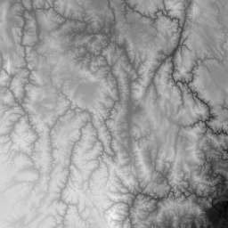
In the spirit of trying new things, rather than tread that worn path again I wanted to try something different for Voxelus.  Rather than generate heightfields from fractals, I wanted to see if I could generate something suitable using real-world Digital Elevation Model (DEM) data.  A little searching turned up the Shuttle Radar Topography Mission (SRTM) data which is available in a variety of resolutions.  Downloading this and writing a little command line tool to load and cut out interesting sections of it enabled me to produce a library of DEM tiles that I could use.

Two examples of DEM patches my tool cut out of the massive SRTM 500m data set

I used a simple height histogram to choose areas where there was a lot of variety in elevation in an effort to make the final result more interesting - although the SRTM 500m data set is hundreds of MB in size, a surprising amount of the Earth's surface is in fact pretty damn flat!

Armed with my library of DEM tiles I needed a way to map them onto my planet.  Mapping 2D squares onto a sphere is however a classically impossible task (ask any cartographer) so rather than being able to make some perfect mapping I instead needed to quilt the surface with overlapping tiles, using as few as possible while ensuring that there were no gaps in between. I also wanted to be able to quilt at various resolutions so I could combine several "octaves" of DEM data in a traditional fractal-esque fashion.

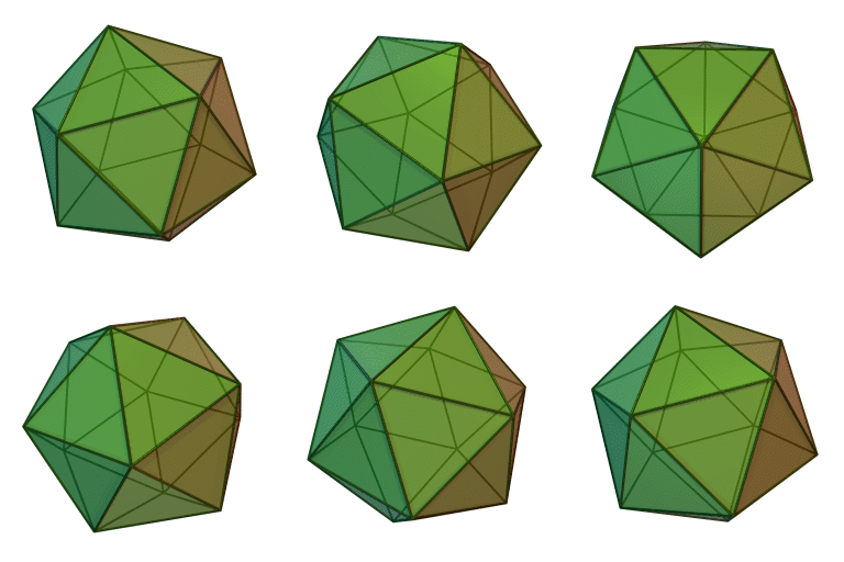
To do this, I based my mapping on an Icosahedron, a regular polyhedron made up of 20 triangles.

Icosahedron (image from Wikipedia)

The key attraction of the icosahedron is that each side is an equilateral triangle producing an even distribution of surface area, and that each side can be recursively subdivided into four smaller equilateral triangles to produce higher and higher detail meshes with the same characteristic.  By normalising the position of the vertices introduced by these subdivisions an increasingly high quality approximation to a sphere is achieved.

To map my DEM tiles onto the sphere I treat each triangle of the icosahedron as representing one tile.  The centre of the tile lies on the centroid of the triangle and extends outwards to cover the triangle completely.  Each tile also has a random rotation around the centroid so to ensure that there are no gaps between the tiles from adjacent faces, the tile has to be twice the radius of the triangles circumscribed circle in size.  There will be considerable overlap around the edges between adjacent tiles but that's all the better to avoid seams.

First "octave" of DEm tiles at primary icosahedron vertices, there are 12 tiles here

One further level of subdivision produces 42 smaller tiles

Subdividing again produces 162 even smaller tiles

These three images are to visualise how the tiles are distributed on the sphere. These examples actually have the tiles at the vertices rather than the triangle centroids but I later switched to the centroids as I thought it gave a better result.  Centroidal tiles produce 20, 80 and 320 tiles at each level respectively.  The tiles here are artificially smaller than final size simply to improve the visualisation.

Expanding the tiles to their correct sizes and repositioning them at the triangle centroids rather than the vertices produces a more accurate result:

Here the individual tiles have been tinted to aid identification and the edges shaded green based upon the weight of their influence at that point.  As you can see the weight of each tile fades off towards it's edges to avoid hard seams and there is no space between them regardless of their orientation to ensure a complete mapping of the sphere.  I've added a simple directional light so the relief from the DEM data can be seen.

Normals from just the basic level #0 data

Here the voxel normals can be seen, note that this is using just the 20 tiles from the level #0 quilting but with a  mountain height of about 500 Km to make detail obvious from such a distance - by comparison Mt. Everest on Earth is just 8.8 Km tall.

Finally here is the same level #0 data with some basic elevation/slope based texturing applied.  Even with just one level of DEM data I am quite pleased with the appearance of the terrain, particularly with the variety of landscape forms in evidence which encourages me that this technique might just be viable.

The coarse 256^3 nature of the data can be quite clearly seen in this image even from this distance so I think starting work on the dynamic resolution subdivision system for closer views might be next on the list of things to tackle.

Sparse Voxel Octrees: A New Beginning

There’s been quite a lot of interest lately in the realtime graphics world to do with Sparse Voxel Octrees (SVOs), so I thought it was about time I had a look at them.  Although I’ve experimented with voxels before, in particular in the Geo project I worked on a few years ago (http://jwhigham.wordpress.com/category/geo) I didn’t really make use of octrees in those cases and more significantly I converted the voxel data to geometry prior to rendering using the classic Marching Cubes algorithm - now generally superseded by better techniques such as Dual Contouring.

Having been down that route before I wanted to try something new so this time I’m endeavouring to render by ray-casting directly against the SVO rather than converting to geometry and rasterising.  I don’t believe that ray-casting (or ray-tracing if you want to consider more than one bounce) is going to replace rasterisation any time soon as the genesis of GPUs has left them understandably specialised for that particular problem and therefore very efficient at it.  I do believe however that when used in conjunction with rasterisation ray casting or tracing is a tool too powerful to ignore and can be an ideal solution for effects such as reflection, refraction, shadows and global illumination that are difficult to simulate with rasterisation, especially at a global scale.

128x128x128 SVO ray-cast on the GPU with simple dot-product lighting

There have been numerous articles published in recent years postulating that rasterisation is dead and raytracing is the next big thing and just as many countenancing the opposite, the truth of course as I see it is somewhere in the middle – both have compelling strengths and weaknesses so surely the best solution is to combine them, using each where best suited to maximise their strengths.

So while it’s technically perfectly possible to convert the voxels to geometry and then intersect rays against the resulting polygonal soup it flies in the face of this belief and doesn’t strike me as a particularly sensible thing to do.  I also want to see if ray casting against the voxel structures directly can help alleviate some of the more challenging problems with geometry based voxelisation, particularly transitions between multiple levels of detail which I struggled with on Geo.  Also like I say, it’s not something I’ve done before which is really reason enough.

128x128x128 Sphere rendered with linear distance filtering

The same sphere rendered with point distance sampling to make the individual voxels clearer

The Aim

Ultimately I would like to recreate my virtual planet out of landscape blocks of varying resolutions right down from global scale viewed from orbit to standing on the surface with reasonable fidelity.  I’ll also need to have a think about how to procedurally generate the data as the flexibility to have full 3D makes the problem far more interesting than just the heightfield used by Isis (http://jwhigham.wordpress.com/tag/isis/) and Osiris (http://johnwhigham.blogspot.co.uk/search/label/Osiris).  I want to avoid if possible having the floating blobs of landscape that plagued Geo’s simplistic 3D noise based solution while still having features that make the 3D nature of the data obvious such as realistic overhangs and caves.

First Steps

As with most new experiments the first thing to do is investigate the existing body of work on the subject, which as I mentioned earlier is quite active at the moment with the dramatic increase in GPU performance and especially their flexibility in recent years.  See the references section at the end for a few links to papers and videos I discovered in my internet SVO safari, it’s by no means an exhaustive list but they are some of the more interesting items I found.

Once I felt I had a sufficient understanding of current techniques I jumped in with both feet and embarked on a bit of coding.  While the aim is to produce a real time GPU based solution my experience of the somewhat patchy tools available for GPU debugging steered me towards producing a reference implementation in C++ on the CPU first.  While it would run far more slowly this would let me debug the code effectively and help me verify that my algorithm and data structures were correct before sending them down to the GPU.
This turned out to be a really useful process and with modern CPUs being pretty powerful themselves (and ray casting being a parallel friendly technique) it was possible to produce a C++ implementation that ran acceptably quickly even in debug builds.  Having it render a quarter resolution version during camera movements and a full resolution one once the camera stopped also helped.

The first technique I attempted was the Laine & Karras one.  While there was sample source code available for this I am of the belief that to properly understand a technique you have to at least have a go at coding it up from first principles so that’s what I did.  After a while though my spider sense started to tell me that storing down to the individual voxel level wasn’t going to be best suited to planetary scales so I switched to the Cyril Crassin paper where he stores an octree down to a certain level then stores bricks of voxels rather than individual ones for the final few levels.

The 16x16x16 grid of voxel "bricks" that make up the actual Octree

The algorithm traverses the octree until it arrives at a suitable level of detail or a leaf node then ray-marches through the chosen brick (8x8x8 in my implementation) to find the accurate intersection.  Written well it's trivial to alter the size of the bricks to compare performance and memory use in different configurations.

This system felt more scalable and better suited to GPU application, plus there were advantages to do with cone tracing through the structure for shadows and global illumination applications that felt worth having available for the future.

Storage

It’s pretty clear that a voxel is a cube shaped blob of space, games such as MineCraft have made the voxel pretty famous these days, but there are a couple of key considerations when rendering them.  Primarily is what each voxel represents, in it’s most simplisitic form a voxel could be considered to be either solid or empty which is easy to understand but limits rendering to producing blocky effects dependent entirely on the size of the voxels in use.  Rather than storing a flag indicating solid or empty with a voxel a better way is to store a distance value representing how far the centre of the voxel is from the surface that is to be rendered.

Under this representation for a landscape voxels above the ground would have increasingly positive values while those underground would have increasingly negative ones.  Rendering the isosurface where the distance is zero would produce the intended surface.  The primary benefit of this scheme is that the distance value can be interpolated accurately between voxels to produce a better approximation of the surface.  The quality of the output is still highly dependent upon the resolution of the data but undersampling artifacts show up as lumpy blobs rather than hard square edges which I think look generally better.

The images below show the progression from highest detail to lowest through the four levels of octree produced by my 128x128x128 noise-blob data.  Note that I've turned off the linear filtering of distance here in all but the final image to make the individual voxels clearer:

The 128x128x128 noise-blob at octree level 4 (highest detail)

The same 128x128x128 blob at octree level 3, each voxel is effectively twice the size

Down to octree level 2 and while the shape remains the detail is largely gone

Finally at the lowest detail level on the crude outline remains.  The 128x128x128 original data  is now effectively being rendered at 16x16x16 resolution.

The same lowest detail level but with linear distance filtering - not a terrible approximation of the blob considering it's only using 1/512th of the data

Normals for shading and procedural texturing can either be pre-calculated and stored in the voxels or calculated at runtime from the gradient of the distance field – empirical testing will show which is faster in practice although my current thoughts are that it's probably better to store higher precision distance values and calculate the normal when needed.  Although many steps are taken through the distance field only the normal at the closest intersection is needed so it only needs to be calculated once before shading.

On top of the distance value there are also other required fields such as material types which I have some ideas for but I’ll get in to that in later posts.

From CPU to GPU

Once I was happy that everything seemed to be working on the CPU I set about converting the code to run on the GPU using a pixel shader.  I toyed briefly with using a compute shader instead as I've heard there are some benefits to converting some traditionally pixel based tasks to the more flexible compute pipeline but I'll save that for a rainy day.  Ray casting seems a natural fit for per-pixel so I'm sticking with a pixel shader for now.

Thankfully as it had always been my intent to run it on the GPU I had written it with that in mind so storing the data structures in textures and moving the code to HLSL was fairly straight forwards.  It did take a few hours to work out the inevitable teething problems compounded by the typically unstable nature of GPU debugging tools but considering what it's doing it didn't take too long.

The benefit of course is that instead of taking a couple of hundred milliseconds to render it now rendered in just a few milliseconds giving me true real-time frame rates.  Being able to dynamically reload the HLSL code and GPU states also meant I could make changes and see the results virtually instantly without having to re-run the program, saving a considerably amount of time.  If you are creating a graphics framework for your own projects I strongly recommend adding this ability!

Two-sphere distance field showing the geometry that is actually sent to the GPU (i.e. 12 triangles).  The back-faces of the cube are rendered instead of the front to allow the viewpoint to move inside the cube and still render

Next Steps

So I have a single sparse voxel octree I can render via ray casting on the GPU complete with surface normals, what's next?  Well the first thing to do is to be able to render multiple SVOs at different points in space, also to have them abut neatly with continuous surface normals so there are no shading seams.

After this I want to add some automatic level of detail control so the tree is traversed less deeply as the voxel bricks become smaller on screen, having this controllable from the user interface would also be useful to allow performance to be measured against visual fidelity.  Next I want to add a new distance generation function to produce blocks that are a bit more landscape-like plus having the materials to go with them.

So, plenty to do then!

References:

As mentioned above, this is a fairly arbitrary collection of some of the links I came across while researching SVOs.  I am sure there are many more so do feel free to report any good ones you find in the comments!

http://www.tml.tkk.fi/~samuli/publications/laine2010tr1_paper.pdf
Efficient Sparse Voxel Octrees – Analysis, Extensions, and Implementation, Samuli Laine Tero Karras, NVIDIA Research

http://en.wikipedia.org/wiki/Sparse_voxel_octree
Sparse voxel octree

http://www.daimi.au.dk/~aquak/MasterThesisKristofRoemisch.pdf
Sparse Voxel Octree Ray Tracing on the GPU, Kristof Römisch, Masters Thesis

http://maverick.inria.fr/Publications/2011/Cra11/
GigaVoxels: A Voxel-Based Rendering Pipeline For Efficient Exploration Of Large And Detailed Scenes, Cyril Crassin, PhD thesis

http://www.youtube.com/watch?v=VpEpAFGplnI
Sparse Voxel Octree (SVO) Demo by Jon Olick

http://procworld.blogspot.co.uk/
Procedural World