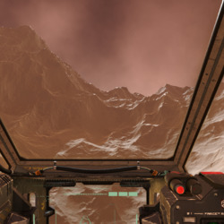
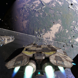
Something that might well be of interest to fellow members of the procedural content generation community is the recently launched KickStarter for Infinity: Battlescape
What started as the ambitious and massively impressive Infinity project many years ago has grown and evolved over time to now underpin the I-Novae technology and it's great to see it hopefully taking a massive step closer to seeing the light of day as a fully functioning commercial production when so many such other such projects wither and fizzle out.
I am happy to back their efforts and hope by posting here that I may in some tiny way spread the word.
Taking a little break from virtual populations I thought it would be interesting to continue the spirit of this project and try out another new technology I've not dirtied my hands with before. Physics (or more specifically mechanics) has been a staple of game development for about ten years now since ground breaking releases such as Half Life 2 and it's popular community modification Garry's Mod in 2004 but even though such technology has appeared in countless products in the last decade I've never actually had to implement it myself so I thought it was about time.
Writing a performant and stable physics system from scratch is a complex and exacting process but fortunately there are a variety of freely available physics solutions that can be leveraged on the PC, one of the most well known of which is the Bullet physics library so that's where I started. My end goal for the initial physics integration was to create a vehicle of some sort that could be driven around on my virtual planet so features pertaining to that objective were the priority. After a little research however I found that the vehicle simulation features of Bullet were quite limited so I looked around for an alternative. On second look I found that the Nvidia PhysX SDK offered a more complete vehicle simulation model so I refocussed my efforts on that.
Although physics can be complex, fortunately PhysX comes with a useful set of samples that were a great aid getting started. Thanks to these it wasn't too difficult to get the SDK linking in and the basic simulation objects for a vehicle up and running. I then hit a wall however as originally I had hoped I could provide some sort of callback to perform the required ray tests for the vehicle against the terrain heightfield but as far as I can tell PhysX simply does not offer this functionality.
What it does provide is a heightfield shape primitive that would normally be a logical fit for vehicle simulation but as these are square and essentially flat while my plant is neither having to make use of them made implementing my vehicle more of a challenge than I had originally intended.
In addition to the problem of mapping square physics heightfield grids to my spherical planet the other major problem is the same one facing virtually every other system involved in planet scale production - namely that of floating point precision. For speed PhysX in line with most real time physics simulation systems operates on single precision floating point numbers by default, but these of course rapidly lose precision when faced with global distances. PhysX can be recompiled to use double precision floating point which would probably sort out the issue but the performance would suffer with such numerically intensive algorithms and as I would like to leave the door open for making more extensive use of physics in the future I didn't really want to go down that route.
The alternative is to establish a local origin for the physics simulation that is close enough to the viewpoint that objects moving and colliding under physics control do so smoothly and precisely even when single precision floating point is used. The key here is that all numbers in the physics simulation are relative to this origin so they never get too big, although for this to work of course the origin itself needs to be updated to stay close enough to the viewpoint as it moves around the planet's surface. As mentioned before my planet is constructed from a subdivided Icosahedron so has as it's basis 20 large triangular patches each of which is subdivided eight times to give 65,536 triangles. As the viewpoint moves closer to the surface these root patches are in turn progressively subdivided each root patch turning into four new patches each made up of the same number of triangles but covering one quarter of the surface area thus increasing the visual fidelity.
My planet is represented by two radii, the Inner Radius which defines how far the lowest possible point on the terrain (the deepest underwater trench say) is from the centre of the planet and the Outer Radius which defines how far the highest possible point is from the centre of the planet (the top of the highest mountain say). Between these two distances lies the planet's crust that is being represented by the terrain geometry. To produce an approximation of an Earth sized planet I am currently using an inner radius of 6360 Km and an outer radius of 6371 Km giving a possible crust range of 11 Km or about 36,090 feet - significantly less than the corresponding distance on Earth were you to measure from the bottom of the Challenger Deep to the top of Mount Everest but I don't have much interest in simulating deep sea environments at the moment so I'm focussing on the more humanly explorable (and visible) portions of our planet for now.
The table below shows the relative size of terrain patches and the renderable triangles they contain at each level of subdivision. As the level increases you can see the number of patches and triangles needed to represent the entire planet grows exponentially, terminating at patch level 18 which would require 90 quadrillion triangles to be rendered!
The patch and triangle sizes and counts for each level of icosahedron subdivision
This Icosahedron topology provides a useful basis for physics origin placement as it naturally divides the planet's surface into discrete units, the decision of which subdivision level to use is all that is necessary. The trade-off here is that using deeper subdivision levels produces more accuracy as it restricts the distance any physics object can be from the origin but necessitates moving the origin more frequently because of this limited range. It also has to be borne in mind that generating heightfield data for the physics system is not instant so the maximum travel speed of any vehicle required to drive upon the ground needs to be restricted such that nearby data can be generated fast enough to be ready by the time the vehicle gets there. In practice I don't think this should be a problem for any real world style vehicle, and fast moving vehicles such as planes can use a different less detailed system.
For now I've chosen to use patch subdivision level 13 as the basis for my physics origin, the reason being that I wanted to obtain a physics heightfield resolution of approximately 1 metre per sample which a 1024x1024 heightfield shape provides for that level (the table shows the patch length of a level 13 patch (L13) is approximately 1 Km). When the physics system is initialised the origin is set to the centroid of the L13 patch under the viewpoint then as the viewpoint moves about and leaves that patch the origin is teleported to the centroid of the new L13 patch above which it now resides. Any active physics objects need to have the opposite translation applied to keep them constant in planet space despite the relocated origin.
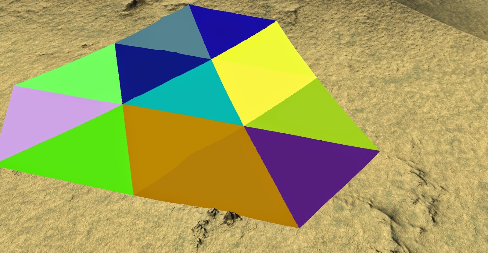
To avoid there being a delay each time the viewpoint moves from one L13 patch to another while the physics heightfield for the new patch is generated as mentioned above the heightfield data for the adjacent patches is pre-generated. Rather than there being eight adjacent patches as you would have for a square grid, the underlying icosahedral topology results in no less than twelve adjacent patches to each central one as shown below:
Colours indicating the 12 patches adjacent to a central one
This means that in addition to producing a heightfield for the patch under the viewpoint twelve more need to be generated ready for when the viewpoint moves. Once this move to an adjacent patch does occur then any new patches not already generated from the twelve adjacent to the new central patch are generated and so on. As all this data generation takes place on background threads the main rendering frame rate is unaffected.
Having a 1024x1024 PhysX heightfield shape for each L13 patch is one thing, but the square essentially 2D heightfield has to be orientated properly to fit onto the spherical planet. This is done by establishing a local co-ordinate system for each L13 patch, the unit vector from the planet centre to the centroid of the patch is defined as the Y axis while the X and Z are produced by using the shortest 3D rotation that maps the planet's own Y axis to the local patch one. Although this does produce a varying local co-ordinate space across the surface of the planet it doesn't actually matter as long as the inverse transformation is used when populating the heightfield - this ensures the heightfields always match the global planet geometry. One final adjustment to make sure the entire planet can be traversed is to modify the direction of gravity with each origin relocation so it always points towards the centre of the planet.
So now there is rolling generation of heightfields as the viewpoint moves around, but even though they are roughly the same size, the 1 Km square heightfields don't really fit onto the triangular patches very well purely because of their shape:
Distant view of the physics heightfields for the centre patch and it's 12 neighbours. The radical difference between the triangular mesh patches and the square physics heightfield shapes causes a huge amount of overlap
A close up of this debugging view highlights how much of the geometry is covered by two or more physics heightfields - computationally inefficient and problematic for stable collisions
This overlap of physics geometry is both inefficient and prone to producing collision artifacts due to the inexact intersections of nearly coplanar geometry. Fortunately PhysX has the ability to mark heightfield triangles as "holes" making them play no part in collisions. Marking any heightfield triangles that fall entirely outside of the owning L13 patch as holes produces a much better fit with minimal overlap between adjacent heightfields.
Distant view of the physics heightfields again but this time quads falling outside of the geometry patch are marked as holes and not rendered showing a much better fit to the underlying mesh topography.
A close up of this second version shows minimal overlay between adjacent physics heightfields
The final step to achieving my goal is the vehicle itself. I'm no artist and don't have a procedural system to create vehicles at the moment so I turned to the internet and found a free 3D model for a suitable vehicle that was licensed for personal use - a Humvee seemed appropriate considering that all driving is off-road at the moment in the absence of roads.
Downloaded Humvee model in Maya. At around 26K triangles it's about right for the balance of detail and real-time performance I want.
This gave me something to render visually but of course the physics model has to be set up appropriately to match with the wheels the right size and in the right place, the suspension travel and resistance set to reasonable values along with the mass of all components and the various drive-train parameters set up to give a suitable driving experience for example.
In total there are quite a few major parameters controlling the physics vehicle model with many more more advanced controls lurking in the background. The all important feel of driving the vehicle relies on the interplay of these many variables so it is important that they can be experimented with as easily as possible to allow tweaking. To this end I put the parameters into a JSON file which can be reloaded with the press of a key while driving around allowing engine power, chassis mass, suspension travel and the like to be altered and the change evaluated immediately for fine tuning.
Example of the JSON for the Humvee simulation model. There are plenty of more advanced parameters the PhysX vehicle model exposes but for my purposes these are sufficient
By making it data driven it also allows me to easily set up different vehicle models simulating everything from fast bouncy beach buggies to lumbering military vehicles or even civilian buses or lorries which sounds like a lot of fun.
Fortunately when playing with all this PhysX includes a really handy visual debugger tool that lets you see exactly what the physics simulation thinks is going on - which can often be quite different to what is being rendered if you have bugs in the mix.
The PhysX Visual Debugger Tool showing the simplified representation of the Humvee represented in the simulation
With PhysX in and working, heightfield shapes set up to collide against and a vehicle to drive hooked up to basic keyboard inputs for steering, acceleration, brake and handbrake I had everything I needed but while fun to drive around I felt it looked somehow wrong...which after a little thought I realised was because the vehicle didn't have a shadow on the terrain. Without this it didn't really feel that it was sitting on the ground more floating some distance above it, and it certainly wasn't clear when it caught air leaping over bumps on the ground.
To fix this I added some fairly rudimentary shadow mapping allowing the vehicle mesh to cast a shadow. There are many techniques to be found for shadow mapping each producing better or worse results in different situations in return for different degrees of complexity. To get something up and running as quickly as possible I implemented plain old PCF shadows using a six-tap Poisson disc based sampling pattern. Even though one of the simplest techniques out there, I was happy with the improvement it provided in making the vehicle feel far more 'grounded':
Without shadows the Humvee looks like it's floating above the terrain somewhere even though it's actually sitting upon it - an effect known as Peter-Panning in shadow mapping parlance
Casting a shadow onto the terrain makes it obvious the vehicle is sat upon the ground while self-shadowing goes a long way to help make it look more part of the scene in general
So that's it, I achieved what I wanted in making a drivable vehicle to tour around my burgeoning procedural planet, as a next step I think some roads might be nice to drive along...
I described in an earlier post my algorithm for placing the
capital city in each of my countries, expanding on that I wanted to gather some
more information about the make up of each country so I can make more informed
descisions about further feature creation and placement.
One key metric is the population for the country as knowing
how many people live in each country is key in deciding not just how many
settlements to place but also how big they should be. Until this is known much of the rest of the
planetary infrastructure cannot be generated as so much of it is dependent upon
the needs of these conurbations and their residents.
World population density by country in 2012. (Image from Wikipedia)
A completely naive solution would be to simply choose a
random number for each country but this would lead to future decisions that are
likely to be completely inappropriate for both the constitution of the
country's terrain and it's geographical location. A step up from completely random would be to
weight the random number by the country's area so the population was at least
proportional to the size of the country but again this ignores key factors such
as the terrain within the country - a mountainous or desert country for example
is likely to have a lower population density than lush lowlands.
To try to account for the constitution of the country's
physical terrain rather than just use the area I instead create a number of
sample points within the country's border and test each of these against the
terrain net. As mentioned in a previous
post, intersecting against the triangulated terrain net produces points with
weights for up to three types of terrain depending on the terrains present at
each corner of the triangle hit. By
summing the weights for each terrain type found on each sample point's
intersection I end up with a total weight for each type of terrain giving me a
picture of the terrain make across the entire country. I can tell for example that a country is 35%
desert, 45% mountains and 20% ocean.
This is of course just an estimate due to the nature of
sampling but the quality of the estimate can easily be controlled by varying
the distance between sample points at the expense of increased processing
time. Given a set number of samples
however the quality of the estimate can be maximised by ensuring the points
chosen are as evenly distributed across the country as possible.
The number of samples chosen for the country is calculated
by dividing it's area by a fixed global area-per-sample value to ensure the
sampling is as even across the planet's surface as possible - currently I'm using one sample per 2000 square kilometres. Once the number is known the area of each
triangle in the country's triangulation is used to see how many sample points
should be placed within that triangle.
Any remainder area left over after that many samples worth of area has
been subtracted is propagated to the area of the next triangle - this also
applies if the triangle is too small to have even a single sample point
allocated to it to make sure it's area is still accounted for.
If a triangle is big enough to have sample points allocated
within it those points are randomly positioned using barycentric co-ordinates
in a similar manner to how the capital cities were placed. There is nothing in this strategy to prevent
samples from adjacent triangles from falling close to each other but in general
I am happy that it produces an acceptably even distribution with a quality/performance
trade-off that can easily be controlled
by varying the area-per-sample value.
So given the proportion of each type of terrain making up a
country how do I turn that into a population value? I assign a number of people per square
kilometre to each type of global terrain, multiply that by the area of the
country then by the weight for that type of terrain to get the number of people
living in that type of terrain in the country then finally sum these values for
each terrain type to get the total number of people in the entire country.
I've produced these people-per-Km2 values largely
by using the real world figures
for population density found on Wikipedia as a basis. Using figures a year or two old, the Earth has an approximate average population density of just 14 people per square kilometre when you count the total surface area of the planet but this rises to around 50 people per square kilometre when you count just the land masses. As shown on the infographic above however the huge variety factors influencing real world population density lead to some areas of the planet being very sparsely populated with only a couple of people per square kilometre while other areas have 1000+. There isn't enough information present in my little simulation to reflect this diversity yet however so I'm currently working with a far more restricted diversity based around the real world mean. The values I am currently using are:
Figures for how many "people" to create per square kilometre for each terrain type
So given the fairly random distribution of terrain on my
planet as it now stands what sort of results drop out of this? Currently the terrain looks like this:
The visual planetary terrain composition, currently the ocean terrain type has a slightly higher weighting so there is more water surface area than any other single terrain type
while making 100 countries produces the figures shown here
Terrain composition for a number of the countries along with their resultant population densities by total area and by landmass area
As can be seen basing the terrain population densities on
real world values has generated a planetary population not too different to our own but as my planet is currently 24% water rather than the 70% or so found on
Earth the actual densities are probably on the low side. The global terrain composition is currently
made up like this:
Proportion of the planet covered by each terrain type and resultant contribution to the planet's population
What is interesting is that the sampling strategy ensures
that the population count properly reflects the proportion of the planet that
is land mass - you can see countries such as Sralmyras which are 32% water have
a lower population density by area of just 13 while Kazilia which is 7% water
has a density of 17 people per Km2.
With a population count my plan is to now use that in
conjunction with the terrain composition profile to derive a settlement
structure for each country so I know how many villages, towns and cities to
create. Watch this space.
I've been somewhat unhappy with the lighting on my terrain for a while now especially the way much of the time it looks pretty flat and uninteresting. It's using a simple directional light for the sun at the moment along with a secondary perpendicular fill light as a gross simulation of sky illumination plus a little bit of ambient to eliminate the pure blacks. Normals are generated and stored on the terrain vertices but even where the landscape is pretty lumpy they vary too slowly to provide high frequency light and shade and with no shadowing solution currently implemented there's not much visual relief evident leading to the unsatisfying flatness of the shading. While I plan to add shadowing eventually I don't want to open that can of worms quite yet so I had a look around for a simpler technique that would add visual interest. I thought about adding normal mapping but the extra storage required for storing tangent and binormal information on the vertices put me off as my vertices are already fatter than I would like. While looking in to this however I came across a blog post by Rory Driscoll from 2012 discussing Derivative Mapping, itself a follow up to Morten Mikkelsen's original work on GPU bump mappng. This technique offers a similar effect to normal mapping but uses screen space derivatives as a basis for perturbing the surface normal using either the screen space derivatives calculated from a single channel height map texture or the pre-computed texture space derivatives of said height map stored as a two channel texture. This was appealing to me not just because I hadn't used the technique before and was therefore interested just to try it out, but also from an implementation point of view I would not have to pre-compute or store anything on the vertices to define the tangent space required for normal mapping saving a considerable amount of memory given the density of my geometry. It also solves the problem of defining said tangent space consistently across the surface of a sphere, a non-trivial task in itself. Thanks to the quality of the posts mentioned above it was a relatively quick and easy task to drop this in to my terrain shader. I started with the heightfield based version as with the tools I had available creating a heightfield was easier than a derivative map but while it worked the blocky artifacts caused by the constant height derivatives where the heightmap texels were oversampled were very visible especially as the viewpoint moved closer to the ground. I could have increased the frequency of mapping to reduce this but when working at planetary scales at some point they are always going to reappear. To get round this I moved on to the second technique described where the height map derivatives are pre-calculated in texture space and given to the pixel shader as a two channel texture rather than a single channel heightmap. The principle here is that interpolating the derivatives directly produces a higher quality result than interpolating heights then computing the derivative afterwards. I had to write a little code to generate this derivative map as I didn't have a tool to hand that could do it but it's pretty straightforward. Although this takes twice the storage and a little more work in the shader the results were far superior in my context with the blocky artifacts effectively removed and the effect under magnification far better.
A desert scene as it was before I started. With the sun overhead there is very little relief visible on the surface
The same view with derivative mapping added. The surface close to the viewpoint looks considerably more interesting and the higher frequency surface normal allows steeper slope textures to blend in
As you can see here the difference between the two versions is marked with the derivative mapped normals showing far more variation as you would expect. The maps I am using look like this:
The tiling bump map I am using as my source heightfield
The derivative map produced from the heightfield. The X derivatives are stored in the red channel and the Y in the green.
Here is another example this time in a lowlands region:
A lowlands scene before derivative mapping is applied
The same scene with derivative mapping.
Particularly evident here is the additional benefit of higher frequency normals where it is the derivative-mapped normal not the geometric one that is being used to decide between the level ground texture (grass, sand, snow etc.) and the steep slope texture (grey/brown rock) on a per-pixel basis. This produces the more varied surface texturing visible in the derivative mapped version of the scene above. Finally, here are a couple more examples, one a mountainous region the other a slightly more elevated perspective on a mixed terrain:
Mountain scene before derivative mapping
The same scene with the mapping applied, the mountain in the foreground shows a particularly visible effect
A mixed terrain scene without mapping
The same scene with the derivative mapping applied. The boundaries between the flat and steeply sloped surface textures in particular benefit here with the transitions being far smoother
To make it work around the planet a tri-planar mapping is used with the normal for each plane being computed then blended together exactly as for the diffuse texture. For a relatively painless effect to implement I am very pleased with the result, the ease of use however is entirely down to the quality of the blog posts I referenced so definitely thanks go to Rory and Morten for that.