Writing a performant and stable physics system from scratch is a complex and exacting process but fortunately there are a variety of freely available physics solutions that can be leveraged on the PC, one of the most well known of which is the Bullet physics library so that's where I started. My end goal for the initial physics integration was to create a vehicle of some sort that could be driven around on my virtual planet so features pertaining to that objective were the priority. After a little research however I found that the vehicle simulation features of Bullet were quite limited so I looked around for an alternative. On second look I found that the Nvidia PhysX SDK offered a more complete vehicle simulation model so I refocussed my efforts on that.
Although physics can be complex, fortunately PhysX comes with a useful set of samples that were a great aid getting started. Thanks to these it wasn't too difficult to get the SDK linking in and the basic simulation objects for a vehicle up and running. I then hit a wall however as originally I had hoped I could provide some sort of callback to perform the required ray tests for the vehicle against the terrain heightfield but as far as I can tell PhysX simply does not offer this functionality.
What it does provide is a heightfield shape primitive that would normally be a logical fit for vehicle simulation but as these are square and essentially flat while my plant is neither having to make use of them made implementing my vehicle more of a challenge than I had originally intended.
In addition to the problem of mapping square physics heightfield grids to my spherical planet the other major problem is the same one facing virtually every other system involved in planet scale production - namely that of floating point precision. For speed PhysX in line with most real time physics simulation systems operates on single precision floating point numbers by default, but these of course rapidly lose precision when faced with global distances. PhysX can be recompiled to use double precision floating point which would probably sort out the issue but the performance would suffer with such numerically intensive algorithms and as I would like to leave the door open for making more extensive use of physics in the future I didn't really want to go down that route.
The alternative is to establish a local origin for the physics simulation that is close enough to the viewpoint that objects moving and colliding under physics control do so smoothly and precisely even when single precision floating point is used. The key here is that all numbers in the physics simulation are relative to this origin so they never get too big, although for this to work of course the origin itself needs to be updated to stay close enough to the viewpoint as it moves around the planet's surface. As mentioned before my planet is constructed from a subdivided Icosahedron so has as it's basis 20 large triangular patches each of which is subdivided eight times to give 65,536 triangles. As the viewpoint moves closer to the surface these root patches are in turn progressively subdivided each root patch turning into four new patches each made up of the same number of triangles but covering one quarter of the surface area thus increasing the visual fidelity.
My planet is represented by two radii, the Inner Radius which defines how far the lowest possible point on the terrain (the deepest underwater trench say) is from the centre of the planet and the Outer Radius which defines how far the highest possible point is from the centre of the planet (the top of the highest mountain say). Between these two distances lies the planet's crust that is being represented by the terrain geometry. To produce an approximation of an Earth sized planet I am currently using an inner radius of 6360 Km and an outer radius of 6371 Km giving a possible crust range of 11 Km or about 36,090 feet - significantly less than the corresponding distance on Earth were you to measure from the bottom of the Challenger Deep to the top of Mount Everest but I don't have much interest in simulating deep sea environments at the moment so I'm focussing on the more humanly explorable (and visible) portions of our planet for now.
The table below shows the relative size of terrain patches and the renderable triangles they contain at each level of subdivision. As the level increases you can see the number of patches and triangles needed to represent the entire planet grows exponentially, terminating at patch level 18 which would require 90 quadrillion triangles to be rendered!
 |
| The patch and triangle sizes and counts for each level of icosahedron subdivision |
For now I've chosen to use patch subdivision level 13 as the basis for my physics origin, the reason being that I wanted to obtain a physics heightfield resolution of approximately 1 metre per sample which a 1024x1024 heightfield shape provides for that level (the table shows the patch length of a level 13 patch (L13) is approximately 1 Km). When the physics system is initialised the origin is set to the centroid of the L13 patch under the viewpoint then as the viewpoint moves about and leaves that patch the origin is teleported to the centroid of the new L13 patch above which it now resides. Any active physics objects need to have the opposite translation applied to keep them constant in planet space despite the relocated origin.
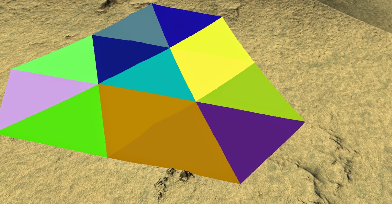
To avoid there being a delay each time the viewpoint moves from one L13 patch to another while the physics heightfield for the new patch is generated as mentioned above the heightfield data for the adjacent patches is pre-generated. Rather than there being eight adjacent patches as you would have for a square grid, the underlying icosahedral topology results in no less than twelve adjacent patches to each central one as shown below:
 |
| Colours indicating the 12 patches adjacent to a central one |
Having a 1024x1024 PhysX heightfield shape for each L13 patch is one thing, but the square essentially 2D heightfield has to be orientated properly to fit onto the spherical planet. This is done by establishing a local co-ordinate system for each L13 patch, the unit vector from the planet centre to the centroid of the patch is defined as the Y axis while the X and Z are produced by using the shortest 3D rotation that maps the planet's own Y axis to the local patch one. Although this does produce a varying local co-ordinate space across the surface of the planet it doesn't actually matter as long as the inverse transformation is used when populating the heightfield - this ensures the heightfields always match the global planet geometry. One final adjustment to make sure the entire planet can be traversed is to modify the direction of gravity with each origin relocation so it always points towards the centre of the planet.
So now there is rolling generation of heightfields as the viewpoint moves around, but even though they are roughly the same size, the 1 Km square heightfields don't really fit onto the triangular patches very well purely because of their shape:
 |
| Distant view of the physics heightfields for the centre patch and it's 12 neighbours. The radical difference between the triangular mesh patches and the square physics heightfield shapes causes a huge amount of overlap |
 |
| A close up of this debugging view highlights how much of the geometry is covered by two or more physics heightfields - computationally inefficient and problematic for stable collisions |
 |
| Distant view of the physics heightfields again but this time quads falling outside of the geometry patch are marked as holes and not rendered showing a much better fit to the underlying mesh topography. |
 |
| A close up of this second version shows minimal overlay between adjacent physics heightfields |
 |
| Downloaded Humvee model in Maya. At around 26K triangles it's about right for the balance of detail and real-time performance I want. |
In total there are quite a few major parameters controlling the physics vehicle model with many more more advanced controls lurking in the background. The all important feel of driving the vehicle relies on the interplay of these many variables so it is important that they can be experimented with as easily as possible to allow tweaking. To this end I put the parameters into a JSON file which can be reloaded with the press of a key while driving around allowing engine power, chassis mass, suspension travel and the like to be altered and the change evaluated immediately for fine tuning.
 |
| Example of the JSON for the Humvee simulation model. There are plenty of more advanced parameters the PhysX vehicle model exposes but for my purposes these are sufficient |
Fortunately when playing with all this PhysX includes a really handy visual debugger tool that lets you see exactly what the physics simulation thinks is going on - which can often be quite different to what is being rendered if you have bugs in the mix.
 |
| The PhysX Visual Debugger Tool showing the simplified representation of the Humvee represented in the simulation |
To fix this I added some fairly rudimentary shadow mapping allowing the vehicle mesh to cast a shadow. There are many techniques to be found for shadow mapping each producing better or worse results in different situations in return for different degrees of complexity. To get something up and running as quickly as possible I implemented plain old PCF shadows using a six-tap Poisson disc based sampling pattern. Even though one of the simplest techniques out there, I was happy with the improvement it provided in making the vehicle feel far more 'grounded':
 |
| Without shadows the Humvee looks like it's floating above the terrain somewhere even though it's actually sitting upon it - an effect known as Peter-Panning in shadow mapping parlance |
 |
| Casting a shadow onto the terrain makes it obvious the vehicle is sat upon the ground while self-shadowing goes a long way to help make it look more part of the scene in general |