Planetary Rings

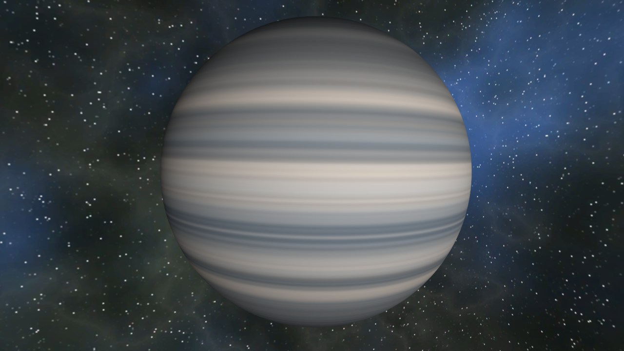
What feels like a logical progression after my recent experiments with gas giant rendering, I thought I would next take a look a adding some rings to my planet, turning it into more of a Saturn than a Jupiter.  Reading up on them, Saturn's rings are a pretty complex structure the formation of which is not completely understood - as ever Wikipedia is a good starting point for information about them. Although they extend from 7,000 to 80,000 Km above the planet's equator they are only a handful of metres thick, being made up of countless particles of mainly water ice (plus a few other elements) from the truly tiny to around ten metres across.

Gas giant with rings as seen at dusk from a nearby planet

My approach for rendering such a complex system is similar in many ways to that for the gas giant itself, rather than ray-tracing though I opted for a more conventional geometric representation of the rings and used a single strip of geometry encircling the planet.  For now the rings are fixed in the XZ plane around the planet’s origin but as the planet itself can have an arbitrary axis in my solar simulation that doesn’t feel like too much of a limitation to be going on with.

Rendering the basic geometry produces this:

Basic ring geometry - a single tri-strip

What’s immediately apparent is once again we fall foul straight away of the polygonal nature of our graphics – although the tri-strip here is a pretty coarse approximation to a circle, no matter how many triangles we add to it we are still going to be able to see straight edges if we get close enough.  Fortunately the solution is simple and by adding a check to the pixel shader to reject pixels that are more than our maximum radius from the planet origin or less than our minimum we immediately get a nice smooth circular ring:

Clipping pixels by distance in pixel shader to produce smooth ring shape

The only trick here is to ensure the vertices of the ring geometry are far enough away from the planet origin that the closest distance of the edges of the triangles is at least the maximum ring radius rather than the vertices themselves being that distance otherwise the outer edges of the ring will be clipped by the geometry:

Vertices (in black) need to be further away than the ring radius to
prevent the ring (in red) being clipped by the triangle edges

A little trig shows this simply to be:


    vertRadius = ringRadius/cos(PI/numSides)


This only applies to the outer edge of the ring as on the inner edge by definition the triangle edges are closer to the centre than the vertices.


Another point to watch is the rings have to of course go both in front and behind the planet itself.  This sounds simple but is made slightly more complex that it first appears as I don't have a Z-buffer available when rendering at the planetary scale due to each planet being rendered in it's own co-ordinate space - they are simply rendered back to front - so they don't share a common Z space that could be used for a Z buffer.  The range of depths would be massive anyway and likely to cause flimmering artifacts.  Add on top of this the fact that planetary atmospheres need to alpha blend on top of whatever is behind them (including the far side of the rings) and a Z buffer isn't really an option.


Instead I render the rings in two passes, the first pass drawn before the encircled planet to provide the bulk of the rings and to allow the planet's atmosphere to alpha blend onto them.  The second pass is drawn after the planet has been rendered and uses an additional ray-sphere and stencil test to only render to the portion of the screen covered by the planet and only where the rings are in front of the planet surface.

Of course one great big slab isn’t very convincing so to get something a bit more realistic I again opted for a similar technique to the gas giant, I took a nice high resolution image of Saturn from the internet and cut out a slice of it’s rings, filtering the result down to a 1x2048 colour ramp texture.

Mapping this texture onto the ring geometry immediately produces something far more pleasing:

Colour ramp mapped onto ring geometry

The colour ramp doesn’t have any alpha information so looks wrong but with a little experimentation it turns out that calculating an alpha value in the pixel shader from the intensity of the colour works pretty well and also softens the inner and outer extremities of the ring:

Colour ramp mapped onto ring geometry with alpha from intensity

As the ring geometry has no thickness however, viewing it from acute angles produces some unsightly single pixel artifacts.  Although in no way scientific, pulling the Fresnel hammer out of the toolbox however makes the effect far less objectionable:

Rings edge-on without Fresnel term showing unsightly aliasing

Rings edge-on with acute Fresnel term - aliasing is reduced at the
expense of increased transparency

Note I’m using a pretty narrow Fresnel band for this purpose otherwise the ring tends to fade out too much of the time.  The number of rings in the effect can be varied with a simple scale value just like for the gas giant.

Changing the scale of the texture look-up to provide fewer, wider rings

More Noise

Although the rings here are pretty decent (largely due to stealing them from a real image I suspect), there is a distinct lack of detail when viewed from anything resembling close up.

Ultimately it would be cool to be able to fade in large numbers of actual meshes to represent the larger ice chunks that make up the rings when the view is near to or actually within the rings, but even without that I thought there was something that could be done to help represent the higher frequency detail these ice particles and ‘ice-asteroids’ present.

As with so many other procedural effects, I decided that a bit of noise would probably add some interest, so I added some code to sample the same noise texture I used for previous effects.  The problem here though is that the particle detail in the rings is very high frequency in the cosmic scale of things but from a purely visual basis I wanted to show variety in the rings from all ranges.

To do this I re-used a trick from the terrain texturing shader where the scale of the texture co-ordinates is calculated on the fly using the partial derivative of the actual texture co-ordinates from the pixel - in this case from the position of the point being shaded on the plane of the rings.  The texture co-ordinates are scaled up or down in powers of two to produce as close to screen size texels as possible - in fact two scales are used by rounding the perfect scale up and down to the closest power of two then blending between these two texture samples to produce a smooth transition.

Ring noise sampled at uniform texel density produces aliasing and tiling at distance

Ring noise sampled at adaptive density to provide more uniform screen coverage without tiling

The texture co-ordinate effect you can see here is somewhat akin to mip-mapping but instead of using a lower resolution version of the texture to represent the same area of surface at a larger distance, I am instead using the same resolution texture to represent a larger area at that distance thereby eliminating the tiling effect often seen with high frequency textures at range.  Unlike mip-mapping it also works in the opposite direction, using the same resolution texture to represent smaller and smaller surface areas as it gets closer to the camera and each texel covers more than one pixel.

Using this signed noise value to lighten or darken each shaded point produces a nice fine grain effect in the rings I hope is vaguely representative of the countless millions of icy particles that in fact make them up.

Rings without noise

Rings with noise to simulate particulate detail

Lighting

As with everything else in my little solar system the rings need to be illuminated by the Sun, this is done simply using standard dot product lighting but the little twist here is to use the noise value from the previous step to slightly perturb the normal uses for the calculation.  This is a gross simulation of the arbitrary facets of the lumps of ice making up the rings being illuminated by the Sun and simply adds a bit of randomisation to the lighting.

A more dramatic effect which adds solidity to the rings is the shadow of the planet cast on to them.  Rather than using shadow mapping techniques this is calculated by doing a ray intersection in the pixel shader from the pixel towards the sun.  To soften the ubiquitous hard edge produced by ray-traced shadows the distance the ray travels through the planet is used to provide a soft edge where the distance is small falling off quickly to solid shadow.  While not strictly physically accurate when classically treating sunlight as a parallel source, I feel it adds to the effect.

Shadow of the gas giant cast onto the rings

Close up of edge of shadow showing the simulated penumbra

Finally the colours in the rings can be remapped again using the same RGB vector system I used before so each final colour component is a dot product of the shader output and the modulation vector passed in to the shader for that channel

Colour re-mapped rings

More drastically colour re-mapped rings :-)

And that's about it.  Any planetary body in my simulation can now have rings of arbitrary radii although it's probably best to not go crazy with them to keep some sense of reality.  Future work for them might include the inclusion of a particle system to provide a sense of thickness as the camera passes through the ring and/or even better a mesh particle system so you can see individual large ice chunks spinning away in space.

For now though, I'll wrap up with another couple of views of my gas giant's rings, comments as always are welcome!

Gas giant with rings from orbit of nearby planet

The same gas giant from nearer the surface of the planet

Gas Giants

Moving on from star rendering in my continuing tour of celestial bodies, I thought it would be interesting to have a go at trying to procedurally render a different type of entity – Gas Giants. 

There are four Gas Giants in our own Solar System, Jupiter, Saturn, Uranus and Neptune each very different from the other, but for my first go at rendering one I decided on the largest of these – namely Jupiter – to see how close to it’s distinctive appearance I could manage at real-time rates.

There is a lot of information available about Jupiter (http://en.wikipedia.org/wiki/Jupiter) and Gas Giants in general (http://en.wikipedia.org/wiki/Gas_giant) on sites such as Wikipedia, again the more I found out about the subject the more interesting it became and I strongly recommend a little background reading if it’s a subject that has any more than a passing interest for you.

Procedural Gas Giant generated and rendered with Osiris

Composite Jupiter image from the Cassini-Huygens probe
(NASA/JPL/Arizona University)

Like stars Gas Giants are conveniently smooth for rendering so I decided to use the same ray-tracing approach that I used for stars described in my previous posts.  This is not only efficient in terms of geometry but also produces lovely smooth spherical surfaces at all screen sizes which is important as I want to be able to fly right down near to the surface of my planets.

I also wanted to be able to produce a wide variety of gas giant effects with only a few input parameters so needed a system that could make interesting visual surfaces with more variation than just their colour.

As seen in the images above, gas giants tend to follow a basic structure of having bands of different coloured material at differing latitudes; these are counter-circulating streams of material called zones and belts and trying to simulate such a major feature seemed like a good starting point.  Using the planet space ‘y’ co-ordinate of the pixel being shaded (essentially the latitude) as a lookup into a colour ramp texture is a nice simple starting point for this effect.  In this case I generated the (1 x 2048) sized look up texture by taking a slice out of the above cassini image of Jupiter and filtering it down to the correct size – this gave me a genuine Jovian colour palette straight off-bat, support for other colours is described below.

Basic colour bands from look-up texture

Using Noise

Already there is a basic sense of a Jupiter like planet but of course it’s way too regular and ordered to give a proper idea of the thick turbulent gaseous atmosphere that makes up so much of this type of world.  Adding some degree of noise to the choice of colour from the ramp texture is an obvious choice in this situation, using the same volume noise texture that I used for the star rendering and combining two weighted channels of two octaves gives a far more interesting result

Noise channel #1

Noise channel #2

Noise channel #3

Noise channel #4

Combined noise

Colour ramp rendered with noise

This looks pretty decent from this fairly distant viewpoint but as the camera moves in towards the surface the pattern loses detail as it’s stretched out over more screen space.  Although the naturally soft nature of the surface detail makes this far less unsightly than it would be on a planet surface with more innate contrast, I thought it could be improved by adding additional octaves of progressively higher frequency noise.

The problem with adding higher frequencies however is that you start to get under-sampling artifacts showing up as sparkly noise in the effect when viewed from too large a distance for that frequency - an almost classic example of shader aliasing.  To avoid this two blend weights are calculated based upon a combination of the distance of the planet from the camera and it’s radius.  These two blend weights are passed to the gas giant pixel shader and used to control the contribution of the upper two bands of noise frequencies.  In this way the higher frequency noise blends in smoothly as the camera nears the surface and fades out as it moves further away.  By choosing the blend distances appropriately the transition is essentially invisible.

Close in to gas giant surface without high frequency noise

Close in to gas giant surface with high frequency noise

Silhouette Edges

The interior of the planet is now looking far more interesting but the silhouette edges are letting it down a bit.  Even at 1280x720 resolution the hard edges are unsightly and without any other anti-aliasing currently in use they jar against the smooth colour graduations of the surface.

While the plan is to add anti-aliasing in the future (either MSAA if performance allows or possibly FXAA) I realised there is something that can be done in the shader itself to improve matters and provide some other desirable effects.  Rather than having a hard edge around the sphere it would be far nicer to have a thin band of alpha pixels fading off around the edge to smooth things out.

Fortunately this is quite simple to do, by using a Fresnel term calculated with a dot product of the surface normal and the ray from the camera to the pixel being shaded the alpha value of the pixel can tend to zero as the surface becomes tangential to the view direction.  The only trick required is to control the amount of Fresnel to use to give a consistent on-screen width of just a couple of pixels for the fall off zone – without this the alpha zone would grow and shrink in size as the camera changed distance.  The Fresnel zone is calculated once in C++ and passed to the shader as a constant.

Planet silhouette edges without Fresnel based alpha - aliasing very evident

Planet silhouette edges with Fresnel based alpha - much smoother

A handy side effect is that by clamping the distance factor a larger fade out zone can be used when the camera nears the planet surface producing a completely non-scientific but rather nice atmosphere effect to soften the horizon at these close-up ranges - this can be seen in the high frequency noise planet close up images above.

Cyclones

Adding noise certainly made the surface of my gas giant more interesting but I wasn’t satisfied, it still wasn’t quite what I had hoped for.  Reading about gas giants and looking at the Cassini image at the top of this post it’s quickly becomes obvious that a primary feature of these planets are large numbers of cyclones and anti-cyclones ranging in size from barely perceptible to ones such as the “Great Red Spot” on Jupiter several times larger than the Earth itself combining to make for a highly turbulent surface.


Modelling planet scale cyclones accurately is a computationally expensive proposition beyond the capabilities of a real time system but there is something that can be done on a purely visual level to give at least a nod towards their presence.  To do this I decided to model a system where a potentially large number of cyclones could be represented as a set of cones emanating from the centre of the planet each with their own radius and rotational strength.  In the pixel shader the point being shaded is tested against this set of cones and should it fall within one is then rotated around that cone’s axis by the cone’s rotational strength scaled by the points distance from the cone’s central axis.


Testing a point against potentially hundreds of cones in the pixel shader is however a whole heap of processing so an efficient way to do so is required.  The method I decided upon was to store the cone information in a relatively low resolution cube map texture that could be sampled using the normal of the planet sphere at the point being shaded to determine which cone the point in question fell within, if any.  This way a single texture read provides all the information without having to iterate over each cone individually in the shader.


The cyclone cube map texture uses an uncompressed 32bit format encoded as follows:

• Red : X component of the unit length axis of the cone that encloses or is closest to this texel
• Green : Y component of the unit length axis of the cone that encloses or is closest to this texel
• Blue : Normalised rotational strength of the cyclone whos cone this texel is affected by
• Alpha : Normalised radius of the cyclone whos cone this texel is affected by, the sign of this value represents the sign of the Z component of the unit length cone axis that is computed in the shader

The format is set up so each byte is interpreted by the GPU as a signed normalised number so the values -128 to +127 are stored in the texture bytes which then arrive in the range [-1, +1] when the texture is sampled in the pixel shader.


The normalised rotational strength of the cyclone and normalised radius values encoded in the texture are scaled in the shader based upon minimum and maximum values passed to it in shader constants.


A little experimentation showed that between 100 and 200 cones of sensible radii could be effectively encoded using a cube map only 128x128 on each side, no two cones being allowed to be within one texel’s worth of angle to avoid filtering artifacts.  A benefit of storing axis and radius information in the cube map rather than actual per-texel offsets is that oversampling artifacts in the texture sampling are avoided as the distance calculations in the shader are operating on the same axial values for every pixel affected by that cone – the down side is that each pixel can only be affected by a single cyclone but I am happy to live with that for now.

Colour coding the pixels based upon the cone axis they are closest to and therefore affected by produces what is essentially a spherical Voronoi diagram of the points where the central axes of each cone penetrates the surface of the sphere

Voronoi diagram showing area of influence of each cyclone

Colour coding the pixels instead with a greyscale value indicating the distance from the central axis of their nearest cone produces the following effect

Position and strength of each cyclone

Clearly indicating the size and position of each cyclone.  Finally, using a combination of this distance value and a global maximum rotational strength supplied to the shader in a constant to rotate each sample point around it’s closest cone axis produces the final cyclone effect:

Final Gas Giant with cyclones

A number of cyclones of different size and strength are easily visible here – it’s not perfect but I think it’s a worthwhile addition that makes the overall effect more interesting.

Colours and Bands

The final step is to allow the shader to produce more varied effects for the potentially large number of gas giants I want my procedural universe to be able to contain.  There are two additional parameters that I’ve added to help support this increase in variety.

The first is a simple scale value that is used to control the mapping of latitude values onto the colour ramp texture.  By increasing the scale the width of the bands can be reduced and their number increased while decreasing the scale of course produces the opposite effect – fewer, wider  bands

Gas Giant with twice as many bands

Gas Giant with half as many bands

The second is a colour remapping post-process for taking the RGB generated by the shader and altering it to add variety.  The manner I thought simplest to do this was to pass three vectors to the shader that are multiplied by the red, green and blue shader colour values immediately before the shader returns.  For example passing (1, 0, 0), (0, 1, 0) and (0, 0, 1) would leave the colour unchanged as the red output is just the red input, the green output just the green input and so on.

Passing different values however completely changes the result allowing the final red, green and blue components that end up on the screen to be an arbitrary mix of those from the shader proper.  Although any range could be used some care needs to be taken to keep the general luminosity in a sensible range or we end up with completely black or pure white planets.  A degree of over-brightening can however produce some funky alien worlds.

Colour remapped gas giant

More dramatically colour remapped gas giant

Further variation could be achieved by using a different noise  texture, different noise octave scales and weights or a different colour ramp texture but for now I think this is sufficient.

Future work

Although the cyclone system was developed for gas giants, there is no reason it couldn't also be applied to other bodies with atmospheres.  The clouds on my Earth style planets for example are currently read from a fBm based cube map but it would be interesting to see how they look with cyclones applied – something else to put on my already lengthy TODO list I think.

This post is already in great danger of suffering from TL:DR so I’ll wrap it up there, my parting shot is this image from the surface of one of the Earth type planets in my solar system that shows the gas giant rising over the horizon.  Always more to do, but I’m quite pleased with the result so far.

Gas Giant viewed from the surface of a nearby Earth-like planet

Solar Temperature

Continuing on from my efforts at rendering stars described in my last post, I decided to have a look at making the visual effect a little more dependent upon actual physical properties rather than simply being a soup of magic numbers that produced an effect I was happy with. Although partially inspired out of curiosity just to see if I could, the ability to produce different star effects is required anyway if my procedural universe is to be more varied that an endless procession of yellow Suns.

Before proceeding I should stress here that my knowledge of solar physics is pretty elementary, being garnered from a bit of Wikipedia browsing and books such as the excellent "Wonders of the Solar System"  so don't call me out if anything I say here is imprecise, incorrect or a blatant lie - I don't pretent to be any kind of expert on this subject.

Conducting even my initial research into the subject however immediately revealed that the physical processes at work in a star are pretty complex, scientists' understanding of even the one at the centre of our own solar system is not completely exhaustive, so picking the correct metric(s) to base my graphical representations upon is as ever a trade-off. The more physically accurate I want the simulation to be the more work is going to be involved and the more complex and therefore slow the code will become. This is a real-time project and the effect has to render in just a millisecond or two so it has to be kept simple, in the end I decided temperature was a pretty obvious measure of how a star looks and of the various temperatures associated with a star (core, surface and corona amongst others) the optical surface temperature seemed like a good fit as it’s largely to do with the observed appearance of the star. Hereafter I’ll refer to this optical surface temperature as simply “temperature”.

The temperature of stars is expressed using the Kelvin scale with the temperature of our own sun being approximately 5700K. (see this page on Effective Temperature or here about Spectrums for more details on this) There are also various classes and classifications used to categorise stars but one of the easiest to understand that I found is the Hertzsprung-Russell diagram which provides a really clear visual representation of the relationship between stars magnitudes/luminosities and their classifications/ temperatures.

(Image from Wikipedia)

For now I’m concentrating on rendering stars from the so called Main Sequence within which our Sun lives, but it would be interesting at a later time to experiment with rendering stars from the white dwarf, sub-giant, giant and super-giant areas. Using temperature as a base then, to render a star using the correct colour therefore I needed a way to convert this temperature value into traditional RGB values I could generate and manipulate in my shaders. It turns out that converting from Kelvin to RGB isn’t entirely trivial but I did find a site that offered a handy look up table that I could use to convert between the two. Rather than perform the conversion numerically in my pixel shader I opted to store this LUT in a tiny texture from which the colour for a given temperature within a given range could simply be read. I actually store 32 levels of each temperature in this 32x32 texture from the base colour up to a blend of a much hotter colour and white to give me something to mix in with the noise texture during rendering.

Tying this into my existing star shader was relatively straightforward, I just had to pass in the temperature of the star as a pixel shader constant then use this along with my noise value to look up the Kelvin to RGB conversion texture . I did at first think something was wrong though as at 5700K my lovely yellow and white "Sun" was rendering as a salmon pink sort of shade - not at all sun-like!

After a little more digging it would appear that along with much of the Earth's populace I've been sold something of a lie for the last four decades! Turns out that our Sun isn't actually yellow at all but is rather that fetching salmon pink I mentioned earlier, it only looks yellow from the Earth (or at times a lovely red when rising or setting) due to the absorption and dispersion of light as it passes through our atmosphere. Presumably TV and Films SFX departments use yellow when rendering the Sun from space for consistency (and so they don’t have to keep explaining why it’s salmon pink)

Anyway, happy that this wasn’t a bug in my shader I had a play around with varying this temperature value I was passing to the shader to change the visible colour of my star which produced what I think are quite reasonable results:

The temperature of each version is overlayed - an interesting fact I wasn't aware of is how the colour passes from red through yellow through white and finally to pale blue with temperature - mentally I had assumed that white would be the hottest, so I learned something there.

Note that it’s not just the colour that’s varying with temperature here, the size and “fuzzyness” of the corona is also increasing as the temperature increases – there’s no particular scientific basis for this, it just felt like hotter stars would be expected to have larger coronas. The magnitude of the screen space ray distortion is also linked to temperature, producing more erratic field movement on hotter stars.

Take a look at the video below to see the transition occurring in real time – there’s no doubt more that could be done for now I think it’s good enough for my purposes: producing a range of interesting stars around which to base my procedural solar systems.

Solar Power

Continuing to take a break from procedural architecture, I've been spending what little time I can spare looking at a completely different scale of challenge - rendering stars!

Although Osiris started out as a project focussed on generating and rendering just a single procedural planet, I've found recently the temptation to expand the scope of the project to encompass an entire procedural universe increasingly difficult to resist and to this end have been reworking many of the internal data storage mechanisms and rendering code to handle this.

Rendering a single planet presents many numerical precision challenges for computation and rendering but an entire universe makes it even more so, fortunately there is a natural hierarchy available to help so within my universe I have galaxies, within my galaxies I have solar systems and within my solar systems I have planets and stars - I'll talk about some of the challenges of navigation in such vast spaces another time but it's stars I want to focus on here.

Rendering stars is a little bit unusual in that much of the time computer graphics are trying to make their subjects look as realistic as possible but with a star that breaks down somewhat - if I were fortunate enough to possess a display capable of truly recreating all possible lighting conditions and smart enough to write code that could accurately render a star I have a feeling that the consequences for anyone and everything in the vicinity of said display would be somewhat undesirable!

Fortunately of course that's not really an issue but the point is that for games as for films and books the problem here is more to create a convincing reproduction of what people imagine a star would look like close up rather than trying to achieve a physically accurate rendition as is desirable for many other real world phenomenons.

Here's what I have come up with so far anyway:

I've focussed on creating something familiar based upon our own Sun (A G2 star according to the Harvard Spectral Classification system) and I'm quite happy with it so far.  It would be interesting to try some other parameters to recreate different classifications of stars - I'll post some screenshots if I get round to that but for now though here's how my glowey yellow ball is made up:

Unlike the planets I've been working with so far, for my purposes stars can be conveniently represented as pure spheres which made me think that using conventional geometry may not be the best way to go about rendering them.  You can certainly get a good approximation of a sphere with triangles but as the body gets larger on screen you inevitably end up with faceted edges unless a truly massive number of triangles are used.  You can also treat the sphere as a 2D disc saving a whole heap of triangles across the surface as only the edges are really significant but you then need some maths to work out the 3D points for the pixels covered by the disc.  Both these systems also suffer from being difficult to incorporate into the corona effect I wanted to achieve so I decided instead to embrace a technology that has a long and distinguished relationship with spheres - namely ray tracing.

By rendering a single screen aligned quad that covers the area of the star on screen, calculating a ray in the pixel shader that passes through the given pixel and then intersecting that ray with the sphere of the star you get a perfect circular edge from any distance and a true 3D point for shading and texturing purposes :

Not the most convincing star perhaps but it shows the ray tracing is working.  Next I wanted to give my star a nice swirly yellow and red pattern but as it's a sphere mapping a 2D texture onto it is a bit troublesome.  Three planar maps could be used and blended together (as I do for the terrain texture) but this tends to suffer from obvious blending artifacts as points move between planes and as the star is a perfect sphere this would account for quite a lot of the area.  A cube map could also be used and generated to avoid seams at the edges (as the skybox does) but as I wanted to animate the effect I was worried about getting enough variation this way.

What I went with in the end was using a 3D volume texture that stored various types and frequencies of noise in it's four RGBA channels.  Although volume textures can be memory hungry, I found that one that was only 64x64x64 in size produced enough variation for what I needed plus it also feels like a really handy texture to have around for future effects.  It's possible to generate noise in a pixel shader using ALU instructions which would save the memory cost but I suspect that my single volume texture read is likely as fast if not faster - although I don't have empirical evidence to back that up at the moment.

One difficulty with using a texture based noise function is that it's essential that the noise tiles smoothly to avoid visual seams where the texture wraps and temporal snapping when the noise is used for animation.  There are a few ways to ensure this but I went with a weighted trilinear blend of eight noise samples for each point in my volume to make sure it blended smoothly from one extreme of the volume to the other.  This also has the benefit of working for any underlying signal generator allowing me to experiment with different noise functions without having to make each of them tile individually.

Using the 3D sphere intersection point to look up into the noise texture, summing and scaling the four different frequencies found there and then mapping the resultant noise value onto a red-yellow-white colour spline produces this effect:

The effect really comes to life though once animation is applied by modulating the co-ordinates used to look up the noise texture over time, see the video below to see this in action.

It's already looking like a big ball of hotness but it's not quite there yet.  To make it look even hotter I add a glow effect by intersecting each pixels ray with not just the inner sphere representing the star's surface, but also with an outer sphere representing the outer edge of the star's corona.  Where the star surface is not hit but the corona is a fresnel term is calculated which is used to control the brightness of that pixel within the corona.  Fresnel is used here so the brightness varies with the angle between the ray from the camera to the intersection point on the corona sphere and the normal of the corona sphere at that point - essentially producing a low brightness where the ray from the camera is nearly tangental to the corona sphere's surface and a high brightness as the ray from the camera become more aligned with the sphere's normal.  In other words the more the ray "looks at" the star the brighter it is which achieves a nice glow around the star's surface:

With a little tweak this technique also works as the view point sinks into the corona filling the screen with progressively brighter colours as you near the surface of the star as one might expect.  To make it more interesting a random jitter is also applied to the radius of the corona sphere to make the effect a bit more lively at runtime.

Another effect which can help make objects look hotter is a touch of screen space distortion. This is an effect commonly used in games and films  where the screen above or around a hot object is given a shimmery effect to simulate the refractive shimmering witnessed in the atmosphere by currents of air with differing temperatures - look into the distance along a road surface on a hot day for example to see this in action.

Where this effect is being applied as a post-process on top of other rendering it can be achieved by taking the frame rendered so far (or in some cases the previous frame for speed) and using that as a source texture in conjunction with perturbed texture co-ordinates to re-render the affected area.  This can be expensive however and doesn't exactly do what I want in this case as I would like to produce some wibble on the surface of the star without affecting the corona.

For this I again dusted off my old ray tracing toolbox and found a suitable technique to achieve my goal.  Rather than render the star's surface once then perturb it afterwards I instead perturb the ray itself using the screen space pixel co-ordinates to index my trusty noise texture prior to testing for an intersection with the star's surface.  This produces a nice heat haze style wobble for the edges and interior of the star's surface but leaves the corona (which is still calculated with the un-perturbed ray) unaffected:

The effect is more obvious the closer you get to the surface so here's a shot from closer up:

and again it's more obvious in motion so see the video below for the full effect.

Finally to produce that desired "OMG My eyes!" look I additively blend on a halo sprite which maxes out some bright areas and produces a nice lens flare effect.  This halos sprite also ensures that the star is still visible when viewed from large distances where rendering the actual surface sphere would cover only a pixel or two if that and produces the sun glow effect when within the atmosphere of a planet.

The size of the halo sprite is also randomly jittered at runtime to make the effect more interesting - nothing scientific about that, it just looks better!

So there you have it, my very own star.  As mentioned above I think it looks best in motion so here's a video I captured to demonstrate just that:

Comments as always are welcome!